Content Defined Chunking (CDC)

Defining Content Defined Chunking

Qu'est-ce que CDC?

Content-Defined Chunking (CDC) is a method of splitting a data stream into variable-sized blocks (“chunks”) based on the content of the data, rather than fixed byte offsets. In CDC, a rolling hash is computed over a sliding window of the data, and a cut-point (chunk boundary) is declared when the hash meets a simple condition (for example, when certain bits of the fingerprint equal a predefined pattern). This approach overcomes the “boundary-shift” problem of fixed-size chunking: if data is inserted or deleted, CDC can still find matching boundaries for the unchanged portions, greatly increasing deduplication effectiveness (FastCDC v2016, v2020).

CDC can detect on the order of 10–20% more redundancy than fixed‐size chunking and is widely used in backup, storage, and content-addressable systems to identify duplicate or similar data at fine granularity.

Unlike fixed-size chunking (FSC), CDC adapts chunk boundaries to the data. A simple example is using a polynomial rolling hash (Rabin fingerprint) on each window of $w$ bytes: if $\mathrm{fp} \bmod D = r$ for some constants $D$ and $r$, then a boundary is marked. In practice, Rabin-based CDC reliably finds boundaries that depend on the data content, but it can be CPU-intensive since it updates and checks the fingerprint at every byte. As a faster alternative, many systems use a Gear rolling hash (introduced in the Ddelta paper and used in FastCDC). A Gear hash maintains a 64-bit fingerprint $fp$ and a static 256-entry table of random 64-bit values $G$. Each new byte $b$ updates the fingerprint as:

$$\mathrm{fp} \leftarrow (\mathrm{fp} \ll 1) + G[b]$$

In other words, the previous fingerprint is left-shifted by 1 bit and a precomputed random value (based on the new byte) is added. Because it shifts out the oldest bit and adds the new byte’s contribution, the Gear hash is a true rolling hash. It uses only three simple operations per byte (one shift, one addition, and a table lookup), so it is extremely fast. By contrast, Rabin requires several shifts, XORs, and multiplications per byte (see Josh Leeb's blog about the 2016 paper). Empirical comparisons note that Gear “uses far fewer operations than Rabin”, making it a good high-speed CDC hash. The Gear table must be filled with random 64-bit values to ensure a uniform fingerprint distribution, but otherwise the algorithm is simple to implement.

Chunk Boundary Detection

To use CDC, one chooses an average target chunk size (for example, 8 KiB) and computes a corresponding bit mask or pattern. A common scheme is: choose $N = \log_2(\text{target\_size})$, then use a mask with $N$ bits set (e.g. $\text{mask} = 0x1FFF$ for 13 bits, giving approximately 8 KiB). In practice, one often uses an “all-zero” check: declare a boundary when $(\mathrm{fp} \,\&\, \text{mask}) = 0$. Under the uniform-hash assumption, each bit of $\mathrm{fp}$ is independently 0 or 1 with probability $1/2$, so using $N$ bits with $\text{mask} = 1$ yields a $1 / 2^N$ probability of a boundary at each byte. Thus, on average, chunks are about $2^N$ bytes long, with an exponential-like distribution of sizes. In code, after updating $\mathrm{fp}$ with each new byte, one checks whether $(\mathrm{fp} \,\&\, \text{mask}) = 0$ and— to avoid tiny chunks—also enforces a minimum chunk size, skipping cut-points until at least $\text{min\_size}$ bytes have been emitted. One also typically enforces a maximum chunk size to cap runaway lengths. Typical parameters might be $\text{min} \approx 32\text{–}128\,\text{KiB}$ and $\text{max} \approx 256\text{–}1024\,\text{KiB}$ for large-file use (e.g. in PyArrow).

When a cut-point is reached, the current chunk is output and the fingerprint resets (often to $0$) to begin a new chunk. In streaming implementations, one can also “roll” out the oldest byte from the fingerprint as the window advances, but in Gear’s simple update formula no explicit removal step is required, since the left shift naturally discards the high-order bit. In effect, Gear continuously “rolls” over a sliding window whose size is determined by the fingerprint width. With an $m$-bit fingerprint and a mask containing $N$ ones, the effective sliding window is on the order of $N$ bits, which roughly corresponds to $N$ bytes if the input bytes are random. For example, using a 13-bit mask in Gear yields an effective window of about 13 bytes, much smaller than a Rabin window of 48 bytes for an 8 KiB target.

Implementation notes: If building your own CDC library, you need to generate a Gear table (for example, 256 random 64-bit values), choose appropriate chunk-size parameters, and implement the update-and-test logic described above. Many libraries (in C, Rust, and other languages) already provide CDC or FastCDC implementations; for instance, the fastcdc crate supports both the original (2016) and updated (2020) algorithms. The mask should be derived deterministically from the target size, for example $\text{mask} = (1 \ll N) - 1$ for $N$ bits. For better consistency, one typically pads or distributes the $N$ ones evenly (as in FastCDC) to enlarge the effective window. The chunking loop then conceptually becomes: update $\mathrm{fp}$, check that the current size is at least $\text{min\_size}$, and then test whether $\mathrm{fp} \,\&\, \text{mask} = 0$.

In summary, a basic Gear-based CDC algorithm can be described as follows: start with $\mathrm{fp} = 0$, and for each input byte $b$,

$$\mathrm{fp} \leftarrow (\mathrm{fp} \ll 1) + G[b]$$

and then apply the following logic:

if current_size >= min_size and (fp & mask) == 0:
    emit_chunk()
    fp = 0
elif current_size >= max_size:
    emit_chunk()
    fp = 0

This simple scheme already yields content-aligned chunks, though it can produce a wide range of sizes if left without further adjustments.

FastCDC (2016) Enhancements

The original FastCDC paper (Xia et al., 2016) built on the basic Gear CDC scheme with three key optimisations to boost speed while retaining high dedup ratio:

1. Enhanced Hash Judgment (Padded Mask): Instead of using a plain mask of $N$ ones, FastCDC pads that mask with additional zeros to effectively enlarge the sliding window. In practice, one generates a larger bit‐width mask (e.g. 48 bits) that still has only $\log_2(\text{target})$ effective ones scattered among them. This makes chunk boundaries harder to meet (so chunks tend to be closer to the average) and increases the hash window. Padding the mask in this way lets Gear achieve almost the same deduplication ratio as Rabin-based CDC while preserving Gear’s speed.

2. Sub-Minimum Cut-Point Skipping: FastCDC observes that the hashing speed bottleneck shifts to the judgment phase once Gear makes hashing cheap. To speed up processing, FastCDC explicitly skips checking the hash for a chunk boundary until a larger minimum size is reached. In other words, rather than checking $(\mathrm{fp} \,\&\, \text{mask}) = 0$ on every byte after the standard 2K or 4K prefix, it waits until the chunk has grown significantly. This “skip” is trivial to implement (just check only after $\text{min\_size}$ bytes) but it can double the speed of chunk finding. The trade-off is a slight drop in deduplication ratio (since small natural cut-points are missed) – on the order of ~10–15% worst-case.

3. Normalised Chunking: To recover deduplication lost by skipping and to avoid extremely small or large chunks, FastCDC introduced “normalised chunking.” This means using two masks (called $Mask_{Small}$ and $Mask_{Large}$) instead of one. For the first part of a chunk (when its current length < desired average), FastCDC applies a larger mask (more 1 bits) so that boundaries are less likely (pushing the chunk to grow). Once the chunk exceeds the target size, it switches to a smaller mask (fewer 1 bits), making boundaries more likely to cut sooner. By selectively biasing the cut-probability based on current length, the algorithm concentrates chunk sizes around the target range. In effect, normalised chunking “normalises” the distribution: most chunks end up between, say, 0.5× and 1.5× the target size. (See image below.) This not only improves deduplication (by avoiding too many tiny/huge chunks) but also enables even larger minimum-size skipping without harming ratio.

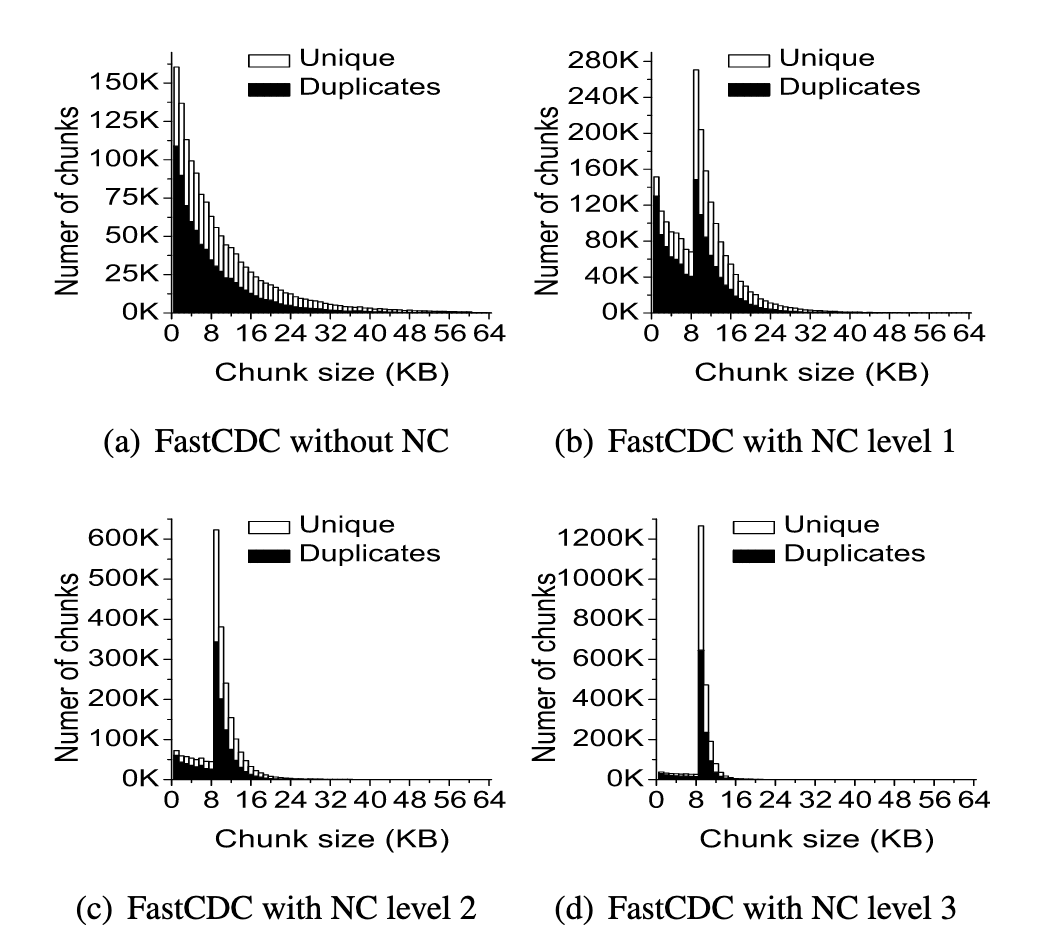
Figure: Chunk-size distribution for un-normalised CDC (with a heavy-tailed spread) vs. FastCDC with normalisation (peaked near target size), from Xia et al. 2016. Normalisation centers the sizes near the mean.

These three techniques made FastCDC much faster than classical Gear CDC or Rabin CDC. The 2016 study showed FastCDC was roughly an order-of-magnitude faster than Rabin-based CDC (up to ~10×) and several times faster than earlier gear/Adler CDCs, while maintaining near-Rabin deduplication ratio.

FastCDC (2020) and Further Optimisations

A follow-up work in 2020 revisited FastCDC and added more refinements. The core algorithm remains Gear-based with padded masks and normalisation, but with additional optimisations for speed:

• Rolling Two Bytes at a Time: The 2020 design introduces an option to process two bytes per iteration. Instead of shifting the fingerprint by 1 and adding $G[b]$ each byte, one can do $(fp \ll 2) + G[b_1] + G[b_2]$ every two bytes (or equivalent). This effectively halves the number of loop iterations and shift operations without changing the logic of cut detection. In practice this “roll-two-bytes” trick can boost chunking throughput ~40–50% while producing the exact same cut positions.

• Implementation Tweaks: Other practical changes include ensuring the same cut points are generated as before while using faster data types (e.g. 64-bit arithmetic) and possibly vectorised hash updates. The overall effect is that the updated implementation (“FastCDC v2020”) yields identical chunk boundaries to the 2016 algorithm but with lower overhead. For example, the Rust fastcdc crate notes that its v2020 module “produces identical cut points as the 2016 version, but does so a bit faster… it uses 64-bit hash values and tends to be faster” (see docs).

• Algorithmic Observations: The 2020 paper also provided analytical guidance on parameter tuning (min/max sizes and normalisation level) to balance speed and deduplication. The normalisation level (how many bits to shift between $Mask_{Small}$ and $Mask_{Large}$) can be tuned: level 0 means no normalisation, higher levels mean a stronger bias toward the average. In general, adding normalisation increases deduplication ratio while skip/min boosts speed. The combination chosen should reflect the application’s priorities.

In short, the “FastCDC 2020” refinements aim to make Gear CDC even faster with minimal loss of chunk-boundary semantics. The key principles (gear hashing, padded mask, skip, normalised split) are the same; the updates allow chunking in fewer operations (two-bytes) and more consistent output across library versions.

Implementation Considerations

Anyone building a CDC library can follow these guidelines:

• Choose Fingerprint Type: Use a 64-bit unsigned integer for the Gear fingerprint to minimize collisions. Pre-generate a 256-entry table of random 64-bit constants for each possible byte (0–255).

• Set Chunk Size Parameters: Decide on $min\_chunk\_size$, $avg\_chunk\_size$, and $max\_chunk\_size$. A typical choice might be avg=64 KiB (target) with min=¼ of that and max=4× that, but values depend on use-case. In PyArrow/Parquet, the default CDC uses avg≈512 KiB, min=256 KiB, max=1024 KiB. These parameters affect both dedup ratio and performance.

• Compute Masks: For a desired average size $M$, set $N = \lfloor \log_2 M \rfloor$. Generate a primary mask with $N$ one-bits (e.g. (1ULL<<N)-1). For normalised chunking, create two masks:

1. $Mask_{Small} = mask \,|\, (1 \ll (N + level))$ (one or more extra ones)
2. $Mask_{Large} = mask \gg level$ (remove bits)

for some $level \ge 1$. The code then uses $mask\_small$ when the current chunk length $< M$, switching to $mask\_large$ once length $\ge M$.

• Loop Logic: Iterate over each byte of the input stream. Maintain a counter of bytes in the current chunk. Update the rolling hash $fp = (fp \ll 1) + G[b]$ for each new byte. Skip any boundary checks until the counter $>= min\_chunk\_size$. Then, in each step, check $(fp \& current\_mask) == 0$. If true (or if counter $>= max\_chunk\_size$), output the chunk boundary, reset the counter and fingerprint (or reinitialise) and continue.

• Normalisation Switch: If using normalisation, at each byte check whether the chunk length has crossed $avg\_chunk\_size$. If not, use the “small” mask for boundary checks; if yes, use the “large” mask. This can be done with a simple if-else each iteration.

• Output Format (Parquet context): In a Parquet/Arrow setting, instead of emitting a raw byte-chunk, one would end the current data page and start a new one. PyArrow’s CDC mode applies these cuts at the level of column values. In practice, this means buffering the column’s serialised values and slicing them into pages when a cut-point is hit (described on the HF blog). The page boundaries are then encoded as Parquet data pages.

• Libraries and Code: Various language bindings exist. For example, the Apache Arrow C++/Python implementation incorporates CDC into its Parquet writer (via the use_content_defined_chunking flag in PyArrow). There are also open-source CDC libraries (e.g. fastcdc in Rust or go-fastcdc in Go) which can be studied or integrated. When writing your own, ensure consistent behaviour by fixing all CDC parameters (mask, table, min/max) identically across runs, so that duplicate data produces identical chunks.

CDC for Parquet Files

In the context of Parquet and data files, CDC is used to allow partial rewrites and deduplication of columns. By default, Parquet writers create fixed row-group boundaries and page sizes. With CDC enabled (use_content_defined_chunking=True in PyArrow), the writer instead splits each column into data pages at content-defined boundaries of the logical column values, before any encoding or compression. This ensures that small edits (like inserting rows or adding columns) only change nearby pages. For example, inserting a row in a column shifts all fixed-page boundaries and would invalidate many pages, but with CDC the chunking adjusts so that most data remains aligned. The Hugging Face Xet layer then sees identical byte chunks and avoids re-uploading unchanged pages.

In practice, using Parquet CDC on a dataset dramatically reduces the volume of changed data. The Hugging Face blog shows that with CDC enabled, adding or deleting rows leads to only ~6–8 MB of new data out of a 96 MB table (versus tens of MB without CDC). The Arrow docs put it like so:

When enabled, data pages are written according to content-defined chunk boundaries, determined by a rolling hash… When data in a column is modified, this approach minimises the number of changed data pages.

To implement something similar, a Parquet writer must collect each column’s values, run the CDC algorithm on their serialised representation, and cut pages accordingly. PyArrow automates this when the CDC flag is set.

Comparison to Other Methods

CDC (especially Gear/FastCDC) should be seen alongside other chunking strategies:

• Fixed-Size Chunking (FSC): Cuts data into equal-sized blocks (e.g. every 64 KiB). FSC is simple and fast but fails badly on insertions/deletions: even a one-byte shift breaks all subsequent alignments. CDC typically finds more matches and captures 10–20% more redundancy than FSC. However, FSC has predictable boundaries (useful in some hardware contexts) and zero overhead.

• Rabin CDC: The classical CDC method uses Rabin (polynomial) hashes. It is robust and well-studied, but slower per byte than Gear. After Gear became popular, research focused on algorithms like FastCDC to match Rabin’s deduplication with much higher speed.

• Content-Defined with Other Hashes: Some implementations use other rolling hashes (e.g. BuzHash, Adler32 variants). Gear and Rabin are the most common in practice for high-performance dedupe. BuzHash (XOR-shift table) can also be very fast but may require careful handling of bit-rotations. In any case, the core CDC idea is the same: sliding window + hash check.

• Normalisation and Thresholding: The FastCDC enhancements effectively produce a hybrid between CDC and fixed-size: by tuning min/max and normalisation, one can approach deterministic sizes. At one extreme, turning min=avg=max yields fixed-size chunking (no dedupe benefit). At the other extreme, very small min and no normalisation yields a highly variable, exponential tail distribution. FastCDC’s goal was to sit in between, benefiting from CDC’s resilience while keeping chunk sizes stable.

Fin

So to recap, Content-Defined Chunking (CDC) is a powerful technique for splitting data based on content rather than at fixed increments into the bytes, enabling fine-grained deduplication and efficient updates (i.e. adding/removing data from a dataset). Gear hash offers a very fast rolling hash for CDC, and FastCDC’s optimisations (padded masks, skip-min, normalisation, double-byte rolling) make it practical for high-speed, large-scale use.

Libraries like PyArrow now expose CDC for Parquet writers, allowing developers to achieve better data transfer efficiency. To implement (or even just appreciate as a user) CDC yourself you should consider the practical concerns discussed here of tuning mask bits, min/max sizes, and normalisation to balance deduplication ratio with performance.